The assumptions, methodology and limitations of a model should be carefully considered for any purpose you apply it to. I haven’t even listed these here, nor otherwise documented the model fully/clearly.Proceed with caution 🙏
Under construction and not yet comprehensively reconciled to ClimateMARGO.jl 🚧
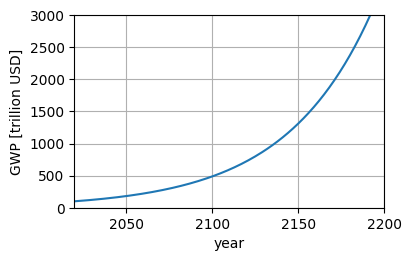
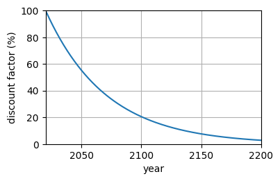
# adapted from ClimateMARGO.jl/examples/default_configuration.jl Henri Drake, MIT licenseusingClimateMARGOusingClimateMARGO.ModelsusingClimateMARGO.UtilsusingClimateMARGO.Diagnosticsinitial_year =2020.0# [yr]final_year =2200.0# [yr]dt =1.0# [yr]t_arr =t(initial_year, final_year, dt);present_year = initial_yeardom =Domain(dt, initial_year, initial_year, final_year);c0 =460.0# [ppm]r =0.5; # [1] fraction of emissions remaining after biosphere and ocean uptake (Solomon 2009)q0 =7.5q0mult =1.0#t_peak = 2100.0#t_zero = 2150.0q =ramp_emissions(t_arr, q0, q0mult, 2300.0, 2300.0); # DN flat 7.5 forverq_effective =effective_emissions(r, q, 0.0, 0.0) # No mitigation, no carbon removalc_baseline =c(c0, q_effective, dt)# These CO$_{2e}$ concentrations drive an anomalous greenhouse effect, which is represented by the radiative forcing# ```math# F_{M,R,G} = a \ln\left(\frac{c_{M,R}(t)}{c_{0}}\right) - G(t)F_{\infty} \, ,# ```# where $a$ is an empirically determined coefficient, $G(t)$ represents the effects of geoengineering, and $F_{\infty} = 8.5$ W/m$^2$ is a scaling factor for the effects of geoengineering by Solar Radiation Modification (SRM).a = (6.9/2.0) /log(2.0); # F4xCO2/2 / log(2) [W m^-2]Finf =8.5;#F_baseline =F(a, c0, Finf, c_baseline, 0.0)ojs_define(c_baseline=c_baseline)ojs_define(F_baseline=F_baseline)# Next, we configure MARGO's energy balance model, which is forced by the controlled forcing $F_{M,R,G}$. The two-layer energy balance model can be solved, approximately, as:# ```math# T_{M,R,G}(t) - T_{0} = \frac{F_{M,R,G}(t)}{B + \kappa} + \frac{\kappa}{B} \int_{t_{0}}^{t} \frac{e^{\frac{t'-t}{\tau_{D}}}}{\tau_{D}} \frac{F_{M,R,G}(t')}{B+\kappa} \, \text{d}t' \, ,# ```# where $T_{0}$ is the initial temperature change relative to preindustrial, $B$ is the feedback parameter, $\kappa$ is , and the timescale $\tau_{D} = \dfrac{C_{D}}{B} \dfrac{B + \kappa}{\kappa}$ is a more convenient expression for the deep ocean heat capacity $C_{D}$.# Default parameter values are taken from [Geoffroy et al. 2013](https://journals.ametsoc.org/doi/full/10.1175/JCLI-D-12-00195.1)'s physically-based calibration of the two-layer model to CMIP5.# Two-layer EBM parametersB =1.13; # Feedback parameter [J yr^-1 m^-2 K^-1]Cd =106.0; # Deep ocean heat capacity [J m^-2 K^-1]κ =0.73; # Heat exchange coefficient [J yr^-1 m^2 K^-1]# Initial condition: present-day temperature, relative to pre-industrialT0 =1.1; # [degC] Berkeley Earth Surface Temperature (Rohde 2013)print("τD = ", round(τd(Cd, B, κ), digits=4), " years\n")# These physical parameters can be used to diagnose the climate sensitivity to a doubling of CO$_{2}$ ($ECS$).print("ECS = ", round(ECS(a, B), digits=4), "ºC") # B=1 gives 3.45# Combined, these parameters define the physical model, which is instantiated by the calling the `Physics` constructor method:Phys =Physics(c0, T0, a, B, Cd, κ, r);# #### 3. Configuring the simple economic model# Economic growth in MARGO (in terms of Gross World Product, GWP) is exogenous $E(t) = E_{0} (1 + \gamma)^{(t-t_{0})}$ and is entirely determined by the growth rate $\gamma$. By default, we set $\gamma = 2\%$.E0 =100.0# Gross World Product at t0 [10^12$ yr^-1]γ =0.02# economic growth rateE_arr =E(t_arr, E0, γ)usingPyPlotfigure(figsize=(4, 2.5))plot(t_arr, E_arr)xlabel("year")ylabel("GWP [trillion USD]")xlim([2020, 2200])ylim([0, 3000]);grid(true)gcf()# Economic damages $D_{M,R,G,A} = \tilde{\beta}E(t) (\Delta T_{M,R,G})^{2} (1 - A(t))$, expressed as a fraction $\tilde{\beta}(\Delta T_{M,R,G})^{2}$ of the instantaneous Gross World Product, increase quadratically with temperature change relative to preindustrial. They can be decrease by adaptation controls $A(t)$. The default value of the damage parameter $\tilde{\beta}$ corresponds to damages of 2\% of GWP at 3ºC of warming.βtilde =0.01; # damages [%GWP / celsius^2]# The total cost of climate controls is simply the sum of their individual costs, each of which follows a parabolic cost function:# ```math# \mathcal{C}_{M,R,G,A} = \mathcal{C}_{M}M^2 + \mathcal{C}_{R}R^2 + \mathcal{C}_{G}G^2 + \mathcal{C}_{A}A^2 \, .# ```# The calculation of the reference control costs $\mathcal{C}_{M}, \mathcal{C}_{R}, \mathcal{C}_{G}, \mathcal{C}_{A}$ are somewhat more complicated; see our Methods in [the preprint](https://eartharxiv.org/5bgyc/) and `defaults.jl` for details. Here, we simply provide their default numerical values, where the costs of mitigation $\mathcal{C}_{M} = \tilde{\mathcal{C}}_{M} E(t)$ and geoengineering $\mathcal{C}_{G} = \tilde{\mathcal{C}}_{G} E(t)$ grow with the size of the global economy and are thus specified as a fraction of GWP, while adaptaiton and removal costs are in trillions of USD per year.ti =findall(x -> x ==2100, t_arr)[1]mitigate_cost_percentGWP =0.02mitigate_cost = mitigate_cost_percentGWP * E_arr[ti] /ppm_to_GtCO2(q[ti]); # [trillion USD / year / GtCO2]print("\nmitigate cost ", mitigate_cost)#print(mitigate_cost)# Costs of negative emissions technologies [US$/tCO2]costs =Dict("BECCS"=>150.0,"DACCS"=>200.0,"Forests"=>27.5,"Weathering"=>125.0,"Biochar"=>70.0,"Soils"=>50.0)# Upper-bound potential for sequestration (GtCO2/year)potentials =Dict("BECCS"=>5.0,"DACCS"=>5.0,"Forests"=>3.6,"Weathering"=>4.0,"Biochar"=>2.0,"Soils"=>5.0)mean_cost =sum(values(potentials) .*values(costs)) /sum(values(potentials)) # [$ tCO2^-1] weighted averageCDR_potential =sum(values(potentials))CDR_potential_fraction = CDR_potential /ppm_to_GtCO2(q0)# Estimate cost from Fuss 2018 (see synthesis Figure 14 and Table 2)remove_cost = (mean_cost * CDR_potential *1.e9) / (CDR_potential_fraction^3) *1.e-12; # [trillion USD / year]adapt_cost =0.115; # [%GWP / year] directly from de Bruin, Dellink, and Tol (2009)geoeng_cost = βtilde * (Finf / B)^2; # [% GWP]# Climate damages and control costs are discounted at the relatively low rate of $\rho = 2\%$, such that future damages and costs are reduced by a multiplicative discount factor $(1 - \rho)^{(t-t_{0})}$.ρ =0.02;figure(figsize=(4, 2.5))plot(t_arr, discount(t_arr, ρ, present_year) *100)xlabel("year")ylabel("discount factor (%)")xlim([2020, 2200])ylim([0, 100]);grid(true)gcf()# These parameters, in addition to a no-policy baseline emissions time-series and present-day control values, define the economic model.Econ =Economics( E0, γ, βtilde, ρ, Finf, mitigate_cost, remove_cost, geoeng_cost, adapt_cost,0.0, 0.0, 0.0, 0.0, # Initial condition on control deployments at t[1] q);# #### A MARGO model configuration is uniquely determined by the parameters defined aboveparams =ClimateModelParameters("rec", dom, Econ, Phys);# ## Instanciating the MARGO climate model# Along with economic and physical model components, the timeseries for each of the four controls must be specified. By default, we simply set these to zero.Cont =Controls(zeros(size(t_arr)) .+0.02, # mitigatezeros(size(t_arr)), # removezeros(size(t_arr)), # geoengzeros(size(t_arr)) # adapt);# The above parameters determine the full configuration of the MARGO model, which is instanced using the `ClimateModel` constructor method:m =ClimateModel( params, Cont);T(m) # T to rec toojs_define(T_m=T(m))ojs_define(T_m_M=T(m; M=true))ojs_define(cost_M=cost(m; M=true))
τD = 239.0108 years
ECS = 3.0531ºC
mitigate cost 0.1664682597045291